Definite Clause Grammars
Writing a parser by hand is one of those exercises that always seems harder than it should be. The grammar fits on half a page; the code somehow doesn’t. Not to worry though - Prolog to the rescue! Prolog has a feature that allows us to do this elegantly: Definite Clause Grammars, or DCGs for short. It’s a small piece of syntax that does a lot. The rest of this post walks through what DCGs are, how they work, and why they’re worth knowing.
Grammars
A grammar is a finite set of rules that says which strings of symbols belong to a language and gives each well-formed string a structural description. More precisely, you write a grammar as four pieces: a set of non-terminals N (the abstract categories), a set of terminals T disjoint from N (the actual symbols that show up in strings), a set of productions P of the form alpha -> beta, and a designated start symbol S drawn from N.
A small example makes this less abstract. Take the language { a^n b^n : n >= 1 }, the strings of some number of as followed by the same number of bs. We can define it with:
N = { S }
T = { a, b }
start symbol = S
P = { S -> a S b,
      S -> a b }
A derivation is a sequence of rule applications starting from the start symbol, where at each step we swap a non-terminal for the right-hand side of one of its rules. Here’s a derivation of aaabbb:
S
=> a S b       (using S -> a S b)
=> a a S b b   (using S -> a S b)
=> a a a b b b (using S -> a b)
aaabbb is in the language because such a derivation exists. aabbb, on the other hand, has no derivation from S, so it’s not in the language.
A second example, closer to what we’ll work with later, is a tiny fragment of English. Here the non-terminals are syntactic categories like noun phrase (np) and verb phrase (vp), and the terminals are actual words:
N = { S, np, vp, det, n, v }
T = { a, robot, kettle, hums, finds }
start symbol = S
P = { S  -> np vp,
      np -> det n,
      vp -> v,
      vp -> v np,
      det -> a,
      n   -> robot,
      n   -> kettle,
      v   -> hums,
      v   -> finds }
A derivation of a robot finds a kettle looks like:
S
=> np vp
=> det n vp
=> a n vp
=> a robot vp
=> a robot v np
=> a robot finds np
=> a robot finds det n
=> a robot finds a n
=> a robot finds a kettle
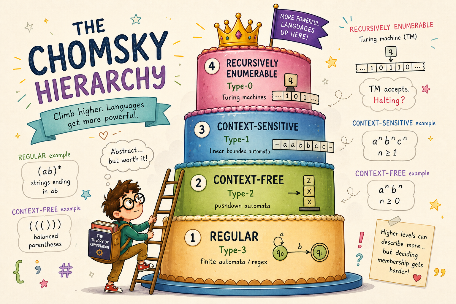
Grammars are usually sorted by what kinds of productions they allow. The Chomsky hierarchy (Chomsky, N., “On certain formal properties of grammars”, Information and Control 2(2): 137-167, 1959) is the standard sorting: regular grammars sit at the bottom, then context-free, then context-sensitive, with unrestricted grammars at the top, and each step admits strictly more languages than the one below. The a^n b^n grammar above is a tidy witness for one of the boundaries: it’s context-free, but a pumping-lemma argument rules out any regular grammar for it, so no finite-state machine will do. DCGs are aimed at the context-free rung by default, though as we’ll see they can climb higher when you need them to.
Context-free grammars and recognizers
A context-free grammar does two jobs at once: it picks out the strings that count as valid sentences of some language, and it pins down how each of those sentences is assembled from smaller pieces. A recognizer cares only about the first job. Hand it a string and it returns a verdict, yes or no, with no further explanation. That’s the whole contract.
From recognition to parsing
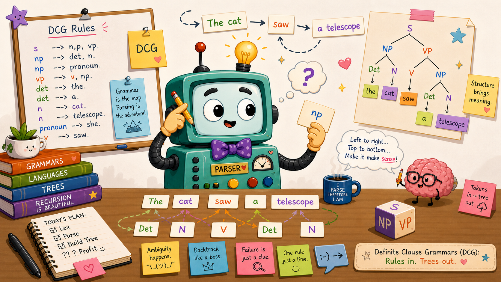
In both linguistics and computer science, we don’t just care whether a string is grammatical. We care why. We want to know its structure, and that’s exactly what a parse tree gives us. A parser is the natural next step beyond a recognizer: instead of returning yes or no, it returns the structure that justifies the answer.
For the English derivation above, the corresponding parse tree records which rule was used at each step:
            S
           / \
         np   vp
        /  \  / \
      det   n v   np
       |    | |  /  \
       a robot finds det n
                     |   |
                     a kettle
The same string can sometimes have more than one parse tree, in which case the grammar is ambiguous. A parser exposes that ambiguity by returning all the valid trees instead of collapsing them into a single yes.
Are natural languages context-free?
A context-free language is one that can be generated by a context-free grammar. Some languages are context-free and some aren’t. For a long time it seemed plausible that the syntax of natural languages might fit inside the context-free family.
Shieber’s 1985 paper on cross-serial dependencies in Swiss German verb clusters (Shieber, S. M., “Evidence against the context-freeness of natural language”, Linguistics and Philosophy 8(3): 333-343, 1985) made that picture harder to defend. The short version is that at least some natural-language constructions can’t be captured by any CFG. The proof filters the relevant Swiss German fragment through a regular language, then uses the pumping lemma to show that the resulting string set still sits outside the context-free family.
That doesn’t mean every natural language is non-context-free. It means the class of natural languages cannot be contained entirely in the CFG family, since it contains at least one language that demonstrably exceeds CFG weak generative capacity. So a grammar for those constructions needs more than context-free rules. When we get to DCGs, we’ll see that the same extra-argument trick that lets us build parse trees also gives us a direct way to push past pure context-freeness.
CFG recognition using append
Turning a CFG into a Prolog recognizer is mostly a copy-paste job once you spot the pattern. Each non-terminal becomes a predicate, each rule becomes a clause, and the input list gets sliced up with append/3 to match the right-hand side of whichever rule we’re trying.
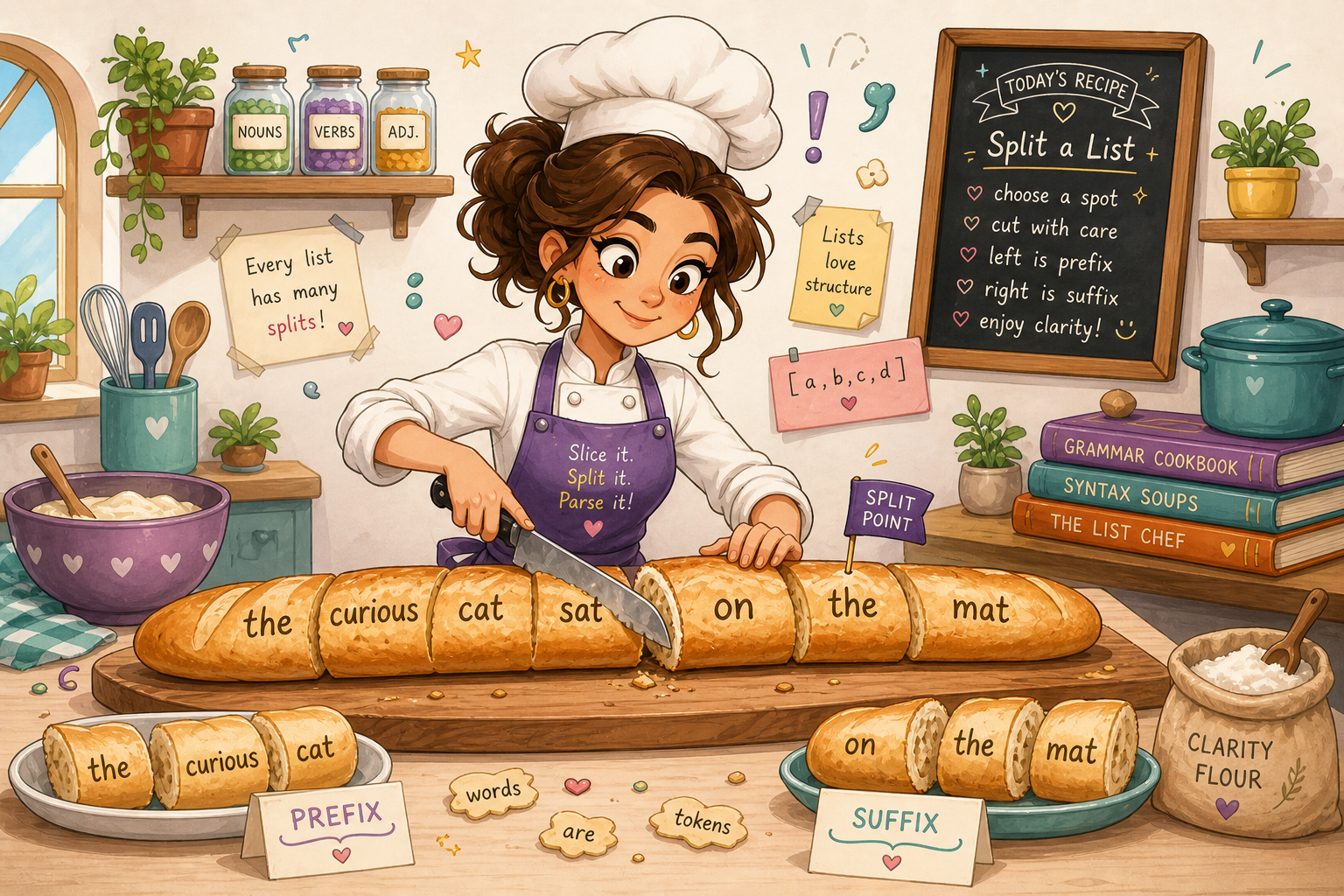
Before the encoding, a quick refresher on append/3. append(L1, L2, L3) holds when L3 is L1 glued to the front of L2. The handy thing is that the same predicate runs in either direction. Call it with L3 bound and the other two unbound, and asking for more solutions enumerates every way of cutting L3 into a prefix and a suffix. That’s a perfect fit for a rule like s -> np vp: let append/3 produce a candidate split, then check that the front piece is a noun phrase and the back piece is a verb phrase.
That’s the whole recipe. Non-terminals turn into single-argument predicates. Each terminal gets a one-element list fact. A binary rule like s -> np vp compiles into a clause with one append/3 call to slice the input in two; a rule with three symbols on its right-hand side needs two splits, four needs three, and so on, either as nested append/3 calls or chained ones. Then each piece gets checked against the right-hand-side categories in order.
Take a small grammar for a fragment of English:
s  -> np vp
np -> det n
vp -> v
vp -> v np
det -> a
n   -> robot | kettle
v   -> hums | finds
The corresponding Prolog program is:
s(S)  :- append(S1, S2, S), np(S1), vp(S2).
np(S) :- append(S1, S2, S), det(S1), n(S2).
vp(S) :- v(S).
vp(S) :- append(S1, S2, S), v(S1), np(S2).

det([a]).
n([robot]).
n([kettle]).
v([hums]).
v([finds]).
We can now ask whether a string is in the language by running a query:
?- s([a, robot, finds, a, kettle]).
true.

?- s([a, kettle, hums]).
true.

?- s([robot, a, hums]).
false.
This is a recognizer in the strict sense: it returns yes or no, no parse tree. To turn it into a parser we’d have to thread an extra argument through every clause to build up the tree as we go.
Two issues with this encoding are worth flagging before we move on. The first is left recursion. A rule like np -> np pp is unremarkable as a CFG, but its Prolog translation np(S) :- append(S1, S2, S), np(S1), pp(S2). is a trap. One of the splits append/3 is willing to produce is S1 = S, S2 = [], which feeds the recursive call to np the very list it was just called on. The next np picks the same clause, gets the same split, and the process repeats. The search has no notion of “we’ve been here before”, so a rule that looks fine on paper turns into a non-terminating loop the moment you try to run it.
The second is efficiency. Every rule with more than one symbol on the right calls append/3 to non-deterministically split the input list, and on backtracking it tries every possible split. For a sentence of any real length and a grammar of any real size, the recognizer ends up exploring a huge number of list splittings, most of which fail immediately. Difference lists, up next, drop the append/3 calls entirely and let unification do the splitting for us.
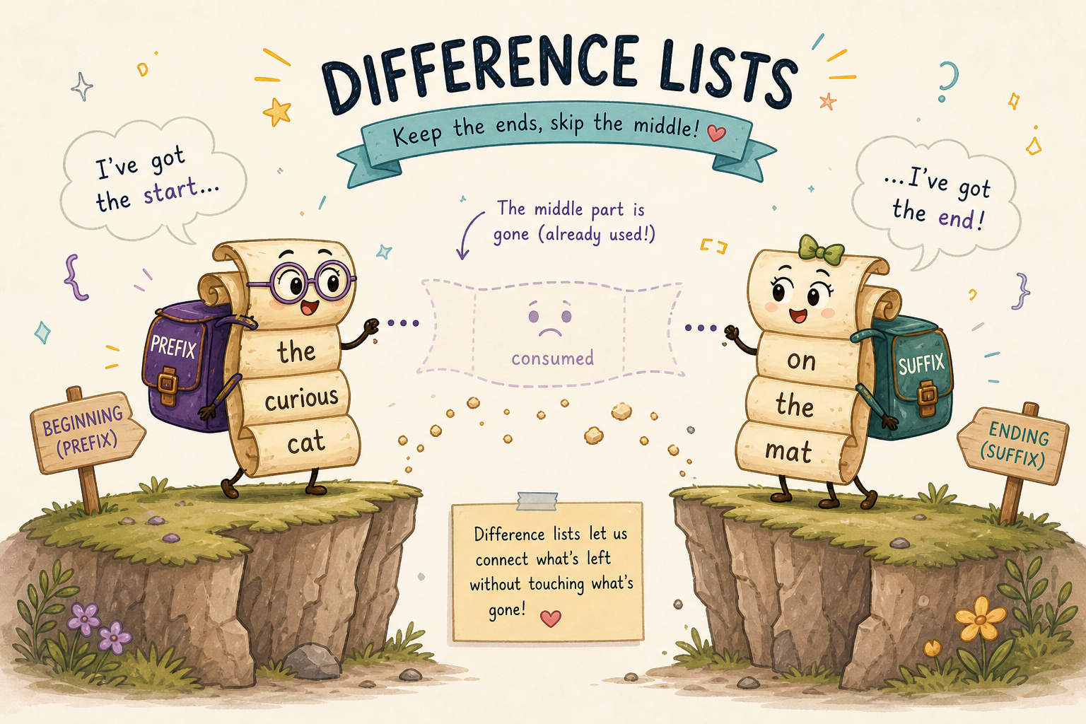
CFG recognition using difference lists
We can do better. The move is to stop thinking of a constituent as its own list and start thinking of it as a slice carved out of a bigger one. Each non-terminal carries two list arguments instead of one: a “before” list and an “after” list. Whatever sits in the gap, meaning the chunk of input the constituent has eaten on its way from the before list to the after list, is the constituent itself.
A few examples in the new notation make this concrete:
[a, robot]is the slice between[a, robot, finds, a, kettle]and[finds, a, kettle]. The pair of lists pins down both ends of the constituent.- An empty constituent is any list paired with itself, like
[finds, a, kettle]and[finds, a, kettle]. Nothing has been consumed. [hums]is the slice between[hums]and[], and equally the slice between[hums, softly]and[softly]. The same constituent can sit at any starting position; the pair of lists is what nails down where.
To say “a sentence is a noun phrase followed by a verb phrase”, we don’t need append/3 to split the input anymore. We just thread the lists: if the noun phrase covers S0 minus S1, and the verb phrase covers S1 minus S, then the sentence covers S0 minus S. The shared variable S1 does the splitting implicitly through unification.
The English fragment from before, rewritten with difference lists, becomes:
s(S0, S)  :- np(S0, S1), vp(S1, S).
np(S0, S) :- det(S0, S1), n(S1, S).
vp(S0, S) :- v(S0, S).
vp(S0, S) :- v(S0, S1), np(S1, S).

det([a | S], S).
n([robot | S], S).
n([kettle | S], S).
v([hums | S], S).
v([finds | S], S).
A query passes the input list as S0 and the empty list as S, which says the whole input has to be consumed:
?- s([a, robot, finds, a, kettle], []).
true.

?- s([a, kettle, hums], []).
true.
Notice that append/3 is gone. Every rule is just a sequence of calls that thread a chain of intermediate lists, and Prolog’s unification fills in the splits as it goes.
The efficiency gap is striking on grammars like this one. Run the sentence [a, robot, finds, a, kettle] against both encodings (as s([a, robot, finds, a, kettle]) for the append/3 version and s([a, robot, finds, a, kettle], []) for the difference-list version) and watch how many list splits each one explores.
The append/3 version, via s(S) :- append(S1, S2, S), np(S1), vp(S2)., has to ask append/3 for every prefix-suffix split of the five-element list. For each candidate it then recurses into np and vp, which fire off their own append/3 calls on the sublists. Most of these splits are doomed and only discover that fact after a few more recursive calls. Combine that repeated split enumeration with Prolog’s depth-first backtracking and the work can grow exponentially in the length of the input, especially once the grammar has any ambiguity to explore.
The difference-list version skips most of that. np(S0, S1) chews through [a, robot] and binds S1 to [finds, a, kettle]; vp(S1, S) carries on from there; nobody had to enumerate splits to find the boundary. The work at each step scales with the length of the constituent that just got matched, and on a deterministic toy grammar like this one the recognizer essentially walks the input front-to-back.
One caveat: that walk-straight-through behavior comes from the grammar, not from difference lists. Underneath, execution is still Prolog’s left-to-right depth-first search with backtracking. Hand it an ambiguous grammar and it will explore alternatives like any other Prolog program. Difference lists buy you cheaper splitting; they don’t buy you linear-time CFG parsing.
The speed comes at a readability cost. The append/3 recognizer reads almost like the grammar itself: each non-terminal takes one argument, and the body of each clause names the right-hand-side categories in order. The difference-list version threads a pair of arguments through every clause, and you’ve got to keep track of which intermediate variable is the output of one call and the input to the next.
The terminal facts also look weirder: det([a | S], S) reads as “consume a from the front of the input and pass the rest along”, which is fine once you’re used to it but it’s noisier than the old det([a]). So we’re trading a compact, declarative encoding that reads like the CFG for a faster but more bookkeeping-heavy one. This is exactly the kind of boilerplate that DCG notation, up next, is designed to hide.
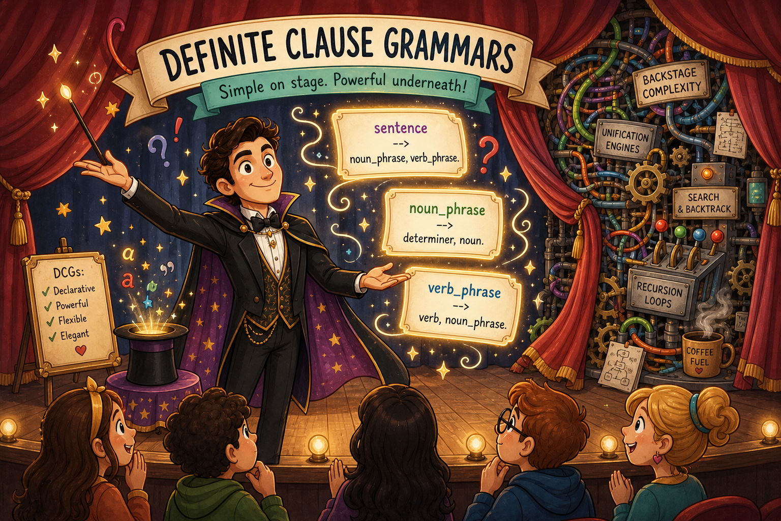
Definite clause grammars
Definite clause grammars (Pereira, F. C. N. and Warren, D. H. D., “Definite Clause Grammars for Language Analysis”, Artificial Intelligence 13(3): 231-278, 1980) are a notation for writing grammars in Prolog that hides the bookkeeping of threading difference-list arguments through every clause, leaving rules that read almost exactly like the original CFG.
The notation uses --> instead of :-, and the two list arguments disappear from the source. Our English example, written as a DCG, becomes:
s  --> np, vp.
np --> det, n.
vp --> v.
vp --> v, np.

det --> [a].
n   --> [robot].
n   --> [kettle].
v   --> [hums].
v   --> [finds].
Compare this to the CFG we started with:
s  -> np vp
np -> det n
vp -> v
vp -> v np
det -> a
n   -> robot | kettle
v   -> hums | finds
The two are basically the same up to punctuation. Each non-terminal on the right-hand side becomes a comma-separated goal, and each terminal is written as a one-element list in square brackets. No list arguments, no S0 and S, no calls to append/3.
Behind the scenes, Prolog translates each DCG rule into exactly the difference-list clause we wrote by hand in the previous section. s --> np, vp. gets rewritten as s(S0, S) :- np(S0, S1), vp(S1, S)., det --> [a]. becomes det([a | S], S)., and so on. The translation is purely syntactic: DCGs don’t add any expressive power on top of difference-list Prolog, they just hide the boilerplate.
To run a DCG, the portable way is to use the built-in phrase/2 (or phrase/3 if you want to expose the leftover list), both of which are standardized in ISO/IEC 13211-1:1995, Information technology - Programming languages - Prolog. phrase(s, L) says “the list L is a sentence and nothing is left over”; in most Prologs it’s equivalent to calling s(L, []) directly on the expanded predicate. Calling the expanded form by hand happens to work in SWI and other common implementations, and you’ll see it in older code, but phrase/2 is the public interface and the form to reach for first:
?- phrase(s, [a, robot, finds, a, kettle]).
true.

?- phrase(s, [a, kettle, hums]).
true.

?- phrase(s, [robot, a, hums]).
false.

?- s([a, robot, finds, a, kettle], []).
true.
Since a DCG rule is just a Prolog clause in disguise, anything we could do in the difference-list version is still on the table. We can add extra arguments to non-terminals to build parse trees or carry agreement features, and we can drop into ordinary Prolog goals inside a rule by wrapping them in { ... }. To build a parse tree, for example, we annotate each non-terminal with an extra argument:
s(s(NP, VP))   --> np(NP), vp(VP).
np(np(D, N))   --> det(D), n(N).
vp(vp(V))      --> v(V).
vp(vp(V, NP))  --> v(V), np(NP).

det(det(a))    --> [a].
n(n(robot))    --> [robot].
n(n(kettle))   --> [kettle].
v(v(hums))     --> [hums].
v(v(finds))    --> [finds].
A query against this grammar returns the structure that justifies the answer instead of just yes or no:
?- phrase(s(Tree), [a, robot, finds, a, kettle]).
Tree = s(np(det(a), n(robot)), vp(v(finds), np(det(a), n(kettle)))).
We’ve moved from a recognizer to a parser without changing the shape of the grammar, just by adding an argument that records what each rule matched. That’s the payoff promised at the start: a notation that stays close to the CFG we’d write on paper, while compiling down to efficient difference-list Prolog underneath.
So far the English we’ve been working with is finite: a handful of words, a fixed set of rules, and a small, finite set of sentences. Real grammars aren’t like this. A noun phrase can contain a prepositional phrase, which contains another noun phrase, which contains another prepositional phrase, and so on without bound. To capture that, a grammar rule has to be allowed to refer to itself, directly or indirectly. That’s what recursion buys us, and it’s where DCGs start to earn their keep. The easiest way to see it is to extend the example.
Recursion and ambiguity
Let’s add prepositional phrases. We extend the lexicon with one preposition (near) and one more noun (window), and we let a noun phrase optionally end with a prepositional phrase. A prepositional phrase is a preposition followed by a noun phrase. As a CFG:
s  -> np vp
np -> det n
np -> det n pp
pp -> p np
vp -> v
vp -> v np
vp -> v np pp
det -> a
n   -> robot | kettle | window
p   -> near
v   -> hums | finds
The recursion is indirect: np can expand to det n pp, and pp expands to p np, so an np can contain a pp, which contains another np, which can contain another pp, and so on. As a DCG, this is just:
s  --> np, vp.
np --> det, n.
np --> det, n, pp.
pp --> p, np.
vp --> v.
vp --> v, np.
vp --> v, np, pp.

det --> [a].
n   --> [robot].
n   --> [kettle].
n   --> [window].
p   --> [near].
v   --> [hums].
v   --> [finds].
The grammar now accepts sentences of unbounded length:
?- phrase(s, [a, robot, finds, a, kettle]).
true.

?- phrase(s, [a, robot, finds, a, kettle, near, a, window]).
true.

?- phrase(s, [a, robot, finds, a, kettle, near, a, window, near, a, robot]).
true.
The second query contains one pp, the third contains two, and we could keep stacking near a ... forever. The grammar itself is still a handful of rules, but the language it generates is infinite.
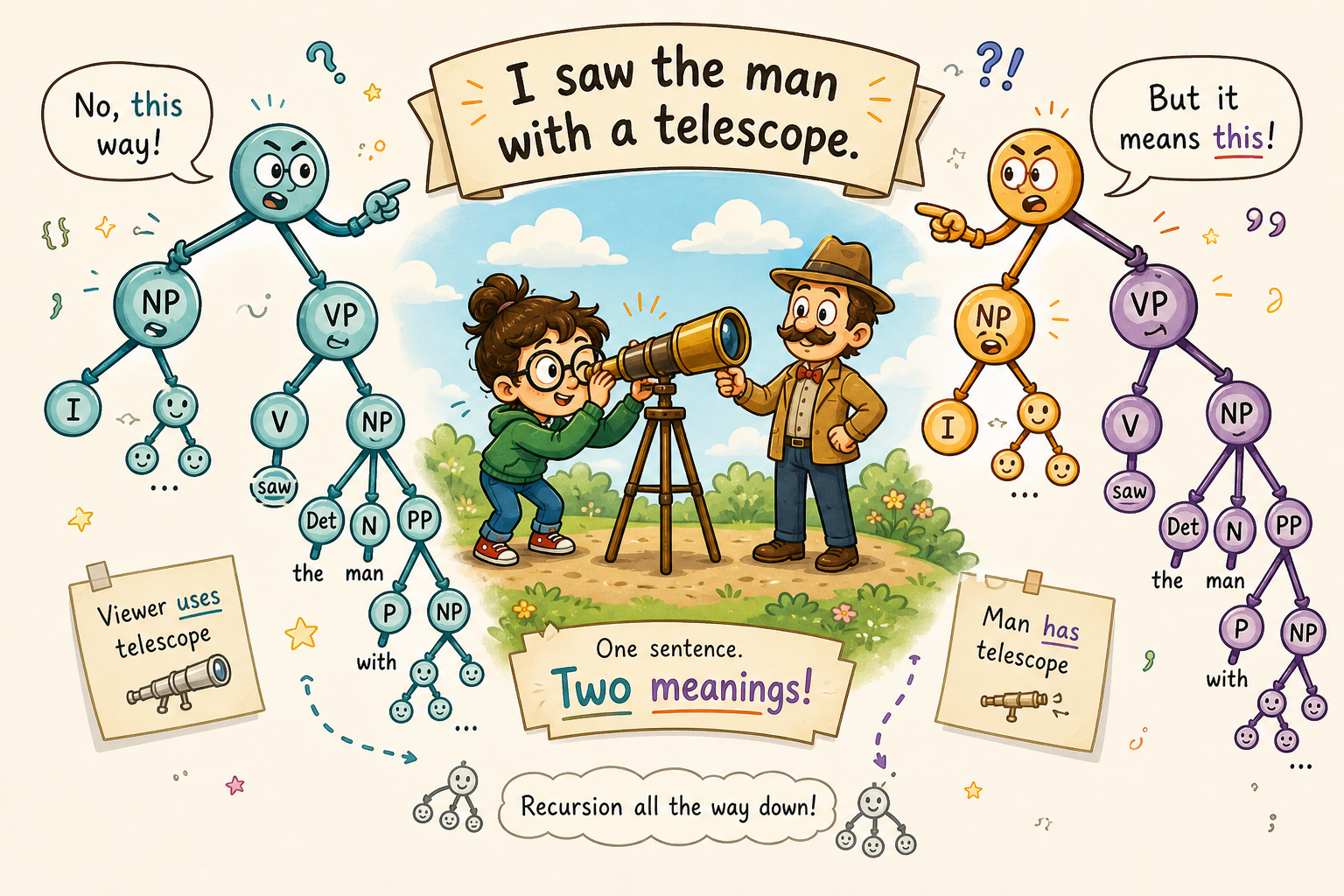
The recursion also drags ambiguity along with it. The sentence a robot finds a kettle near a window has two valid parses: one where the prepositional phrase modifies the object noun phrase (a kettle near a window, the kettle in question is the one by the window), and one where it modifies the verb phrase (the finding is what happens near the window, regardless of where the kettle started out). If you thread a Tree argument through np, vp, and the new pp rule the way we did before, a query on this sentence returns both trees as you ask for more solutions. That’s the behavior we want from a parser staring at a genuinely ambiguous input.
Summary
We started with grammars in the abstract, then walked through three ways to encode the same small English fragment in Prolog. The append/3 version was easy to read but wasteful. The difference-list version recognized the same sentences with much less splitting, at the cost of extra bookkeeping. DCG notation gave us the best of both: rules that look like the grammar on paper, but compile down to the difference-list machinery underneath.
That notation also leaves room to grow. Extra arguments turn recognizers into parsers, thread features or semantic representations through the grammar, and let DCGs reach beyond pure context-free rules when the problem calls for it. Recursion gives us infinite languages, and ambiguity falls out naturally as multiple valid parses.
The catch is that DCGs still run like Prolog. Goal order matters, left recursion can loop, and a grammar that parses neatly may behave differently when used for generation. Once you know to watch for those edges, DCGs are a remarkably compact way to write grammars that stay close to the formalism while still living inside a real programming language.
Comments