Autoregressive Decoder-Only Transformers
If you have used ChatGPT, Claude, or Gemini, the core text-generation model behind those products is usually some scaled-up version of an autoregressive decoder-only transformer. Production stacks differ in the details (multimodal inputs, tool and runtime layers, plenty of architecture details that aren’t public), but the core recipe at the heart of generation is the same: read your prompt, predict the next token, append it, and do it again. One token at a time, until either the model emits an end-of-text token or the runtime cuts it off (max length, a configured stop sequence, a tool-call boundary, or a policy stop).
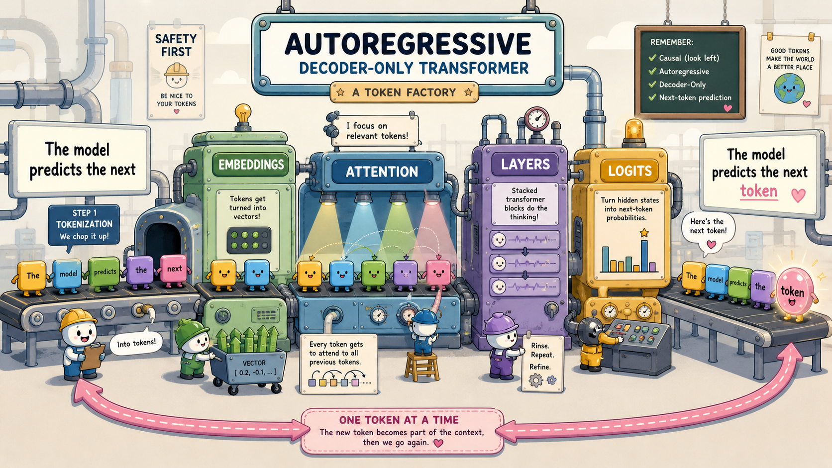
Under the hood, all of this is math. Your text gets chopped into tokens, the tokens get turned into vectors, and from that point on everything the model does is linear algebra: matrix multiplications, dot products, additions, and a couple of nonlinear “squashing” steps like softmax (which turns scores into probabilities) sprinkled in. The “intelligence” we see is the output of billions of learned numbers being multiplied against the numbers that represent your prompt. There is no hand-written grammar, no fact database wired into the core model, no if-statements about syntax.
A quick note on the two models I’ll bounce between. For tokenizer examples I’ll use cl100k_base, the GPT-4-era tokenizer, because it’s a widely-used modern reference. For everything that requires actually peeking inside a model (embeddings, attention weights, hidden states, logits) I’ll use GPT-2 small, because it’s small enough to load on a laptop and Hugging Face exposes every internal tensor. The specific token IDs differ between the two, and modern models vary in details like position encodings, normalization, and attention variants, but the broad shape of the pipeline is the same.
This post grew out of a two-part tech talk I gave on the same material. If you’d rather flip through the slides, you can grab them here: part 1 (tokens, embeddings, attention) and part 2 (layers, logits, generation).
Tokens: How the Model Sees Text
Words Are Not the Unit
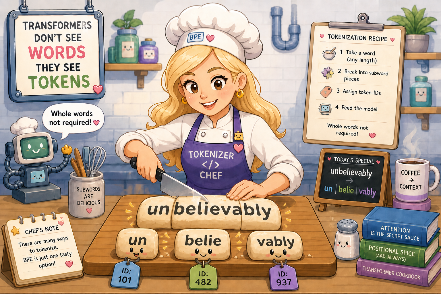
Transformers don’t actually see words. They see tokens, which are usually subword pieces. The word “unbelievably” doesn’t get fed in as one chunk; the GPT-4-era tokenizer splits it into “un”, “belie”, and “vably”, and each piece becomes its own integer ID.
import tiktoken

enc = tiktoken.get_encoding("cl100k_base")  # used by GPT-4-era text models; GPT-4o uses o200k_base
ids = enc.encode("unbelievably")
pieces = [enc.decode_single_token_bytes(i).decode() for i in ids]
print(list(zip(pieces, ids)))
# [('un', 359), ('belie', 32898), ('vably', 89234)]
Those integer IDs are the only thing the rest of the model ever sees. From here on, “the model reads the prompt” really means “the model is handed a list of integers”.
Same Token ID, Different Meanings

Take the sentence “The bank by the river was steep, but the bank approved her loan.” Both occurrences of “ bank” get the exact same token ID. The tokenizer does not know or care that one is a riverbank and the other is a financial institution. It is simply a lookup table.
enc.encode(" bank")  # -> [6201]
# Always the same id for " bank" in cl100k_base. GPT-2's r50k_base happens to use 3331.
(That leading space in " bank" is not a typo. Modern tokenizers treat the space before a word as part of the token itself, so “bank” at the start of a sentence and “ bank” in the middle of one are different tokens with different IDs. I’ll keep the leading space whenever I’m referring to the “bank” that appears mid-sentence in our running example.)
That ambiguity is not a bug. It’s the entire reason the rest of the model exists. Attention, which we’ll get to in a few sections, is one of the main mechanisms that pulls “ deposited” and “ cash” into “ bank”’s representation so the model can lean toward the financial kind. It doesn’t act alone: many other moving parts inside each layer (residual connections, more linear projections, and the per-token feed-forward network inside every layer) all contribute to the final representation. We’ll cover residuals and the projection layers as we get to them; the feed-forward network is its own beast and gets its own follow-up post.
Different Tokenizers, Different Splits
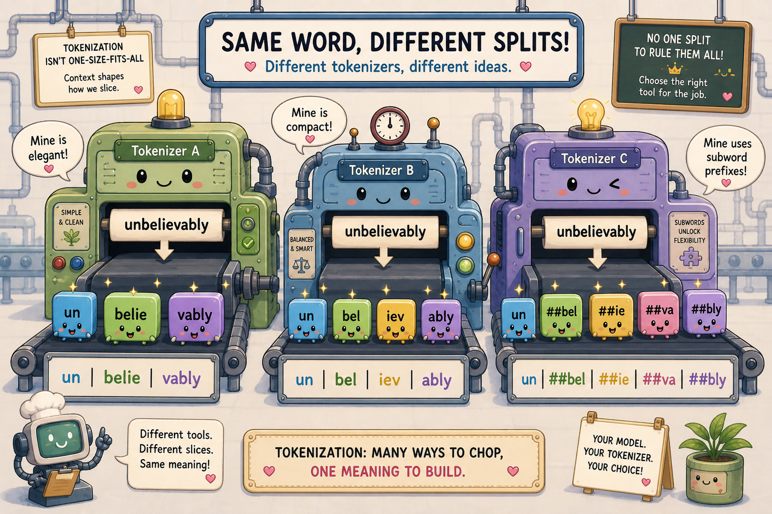
Tokenization is also model-specific. The same string gets sliced differently depending on which tokenizer you use, because each one was trained on different corpora, with different vocabularies, and using different tokenization algorithms.
from transformers import BertTokenizer

cl100k = tiktoken.get_encoding("cl100k_base")  # GPT-4-era
gpt2   = tiktoken.get_encoding("r50k_base")
bert   = BertTokenizer.from_pretrained("bert-base-uncased")

text = "unbelievably"
print(cl100k.encode(text))   # 3 tokens: un | belie | vably
print(gpt2.encode(text))     # 4 tokens: un | bel | iev | ably
print(bert.tokenize(text))   # 5 tokens: un | ##bel | ##ie | ##va | ##bly
cl100k_base uses byte-pair encoding (BPE), a common trick in modern tokenizers. The short version: start with raw bytes, look at a big pile of training text, and repeatedly merge whichever adjacent pair of pieces shows up together most often into a new single piece. Do that thousands of times and you end up with a vocabulary where common words (“the”, “and”) are one piece and rare words (“unbelievably”) get split into a few common subwords. Because the merges are recorded, byte-level BPE schemes are reversible, so you can always recover the original bytes from the IDs. But the choice of where to cut is baked in at training time and biased by whatever text the tokenizer was fit on. Everything downstream operates on these IDs, which means the model inherits whatever tokenization assumptions were made up front.
Takeaway: tokenization is a discrete, language-biased preprocessing step that turns text into integers. The model never sees your characters, only the IDs.
Embeddings: Tokens Become Vectors
One-Hot Is Useless
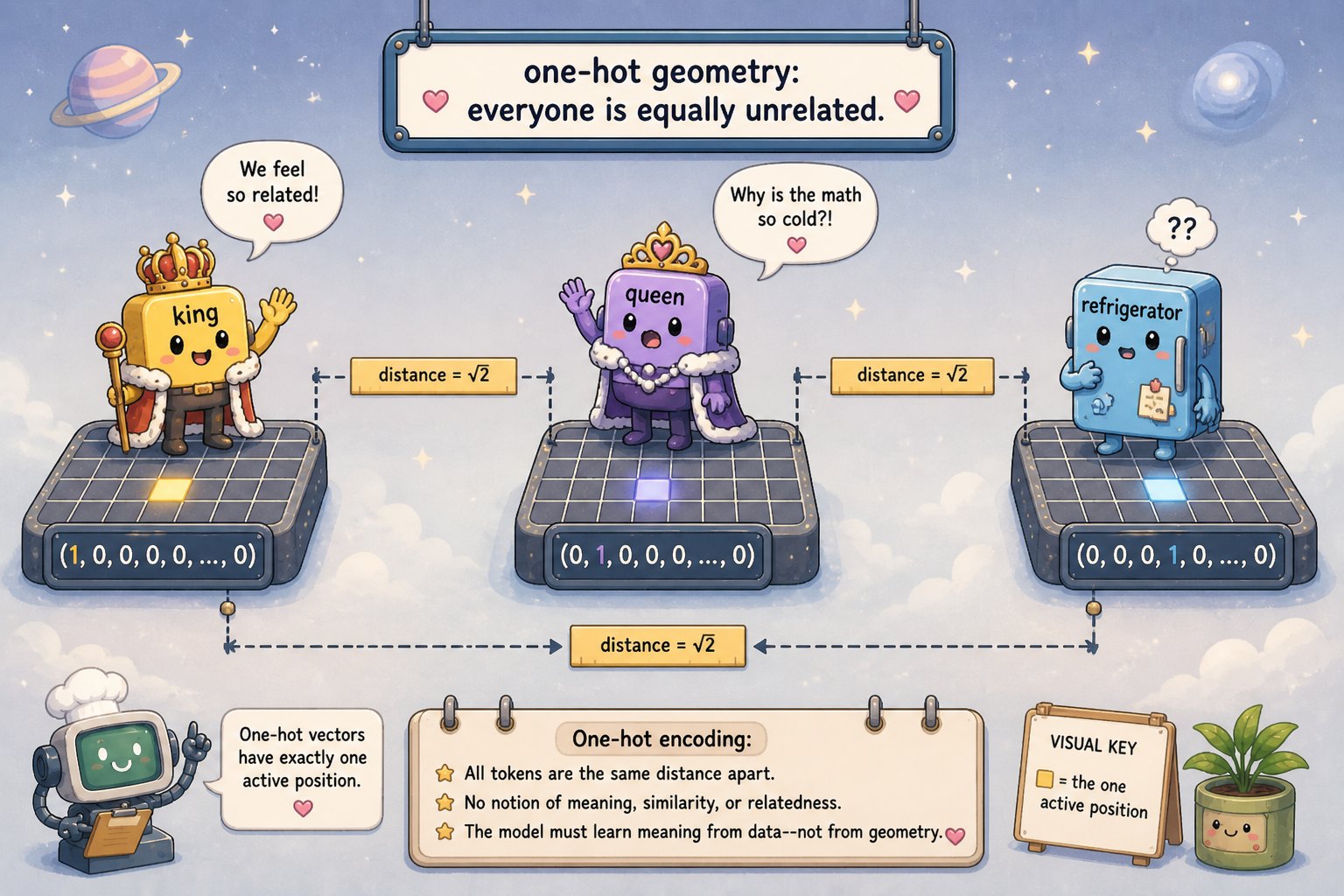
The simplest way to turn a token ID into a vector is one-hot encoding: pick a vector as long as the vocabulary, set the slot for your token to 1, and leave everything else at 0. It’s an unambiguous way to represent “this token and no other”, but it’s a terrible way to represent meaning.
The problem is geometry. Take a sample 5-word vocabulary with king, queen, and refrigerator at positions 1, 2, and 3:
king         = [0, 1, 0, 0, 0]
queen        = [0, 0, 1, 0, 0]
refrigerator = [0, 0, 0, 1, 0]
The dot product is just the sum of elementwise products:
king . queen        = 0*0 + 1*0 + 0*1 + 0*0 + 0*0 = 0
king . refrigerator = 0*0 + 1*0 + 0*0 + 0*1 + 0*0 = 0
king . king         = 0*0 + 1*1 + 0*0 + 0*0 + 0*0 = 1
Every distinct pair scores zero. The 1 only shows up when a token is dotted against itself. There is no way for this geometry to express “king is closer to queen than to refrigerator”, because as far as the math is concerned, they are all equidistant.
import numpy as np

vocab_size = 100_277  # cl100k_base
# "king" and "queen" are single cl100k_base tokens, but "refrigerator"
# actually splits into [ref, riger, ator]. We use the first subtoken
# (1116 = "ref") here so the executable snippet stays a pure single-token
# comparison. Treat it as a sample, not a faithful "refrigerator".
king_id, queen_id, fridge_id = 10789, 94214, 1116

def one_hot(idx, n):
    v = np.zeros(n); v[idx] = 1.0; return v

king   = one_hot(king_id,   vocab_size)
queen  = one_hot(queen_id,  vocab_size)
fridge = one_hot(fridge_id, vocab_size)

print(king @ queen)   # 0.0
print(king @ fridge)  # 0.0
print(king @ king)    # 1.0
So we need something denser, where similar tokens end up near each other in space.
Learned Embedding Vectors
The fix is to give every token ID its own learned vector. Stack all of those vectors as rows of a big matrix E, and “embedding lookup” is just picking row id. In GPT-2 small, that matrix is 50,257 rows by 768 columns, so each token gets a 768-dimensional vector.
Here’s the idea with a sample 6-word vocab and 2D embeddings:
E = [[0.1, 0.9],   # id 0: I
     [2.0, 1.1],   # id 1: deposited
     [2.1, 0.1],   # id 2: cash
     [0.0, 1.2],   # id 3: at
     [0.2, 0.0],   # id 4: the
     [1.0, 2.0]]   # id 5: bank

E[5] = [1.0, 2.0]  # bank
A nice equivalent view: indexing row 5 of E is the same as one_hot(5) @ E. Both pictures matter. At small scale it feels like a lookup, but in matrix form it’s a single linear map. That linear-map view is what makes weight tying natural at the output: the same matrix can be transposed and reused as the unembedding when we go from the final hidden vector back to logits over the vocabulary. GPT-2 ties its input embedding and output unembedding this way; not every model does.
from transformers import GPT2LMHeadModel, GPT2TokenizerFast

tok = GPT2TokenizerFast.from_pretrained("gpt2")
model = GPT2LMHeadModel.from_pretrained("gpt2")

W_e = model.transformer.wte.weight.detach().numpy()  # (50257, 768)
bank_id = tok.encode(" bank")[0]
bank_vec = W_e[bank_id]
print(bank_vec.shape)   # (768,)
Meaning as Geometry
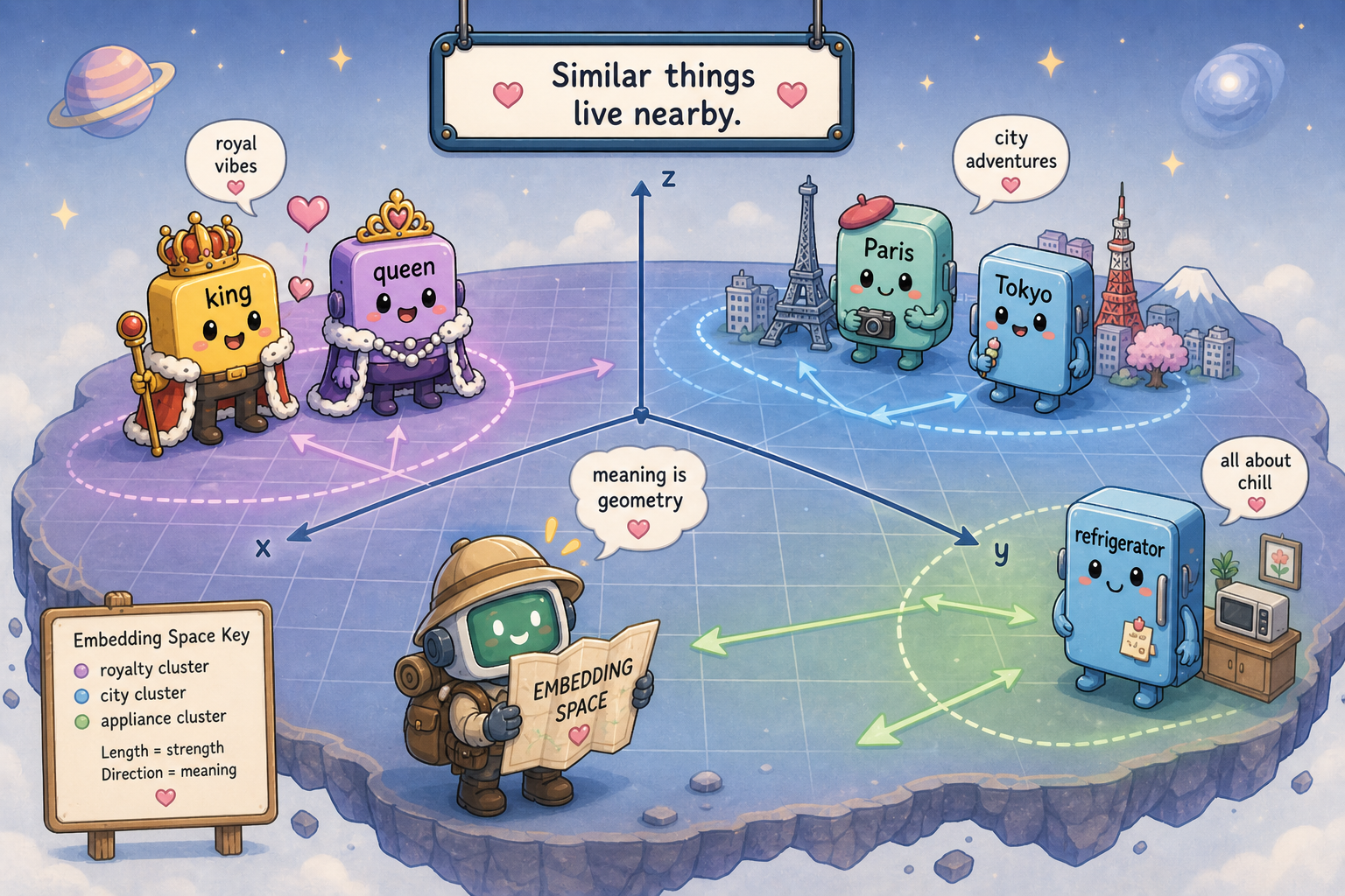
Once tokens live in a dense vector space, the geometry can actually carry meaning. In standalone embedding models like GloVe, cosine similarity between learned vectors reflects relatedness, and some analogies even fall out as vector arithmetic.
import gensim.downloader as api

glove = api.load("glove-wiki-gigaword-300")

glove.most_similar(positive=["king", "woman"], negative=["man"], topn=1)
# [('queen', 0.6713)]

glove.most_similar(positive=["paris", "japan"], negative=["france"], topn=1)
# [('tokyo', 0.8179)]
It’s worth not reading too much into this. Analogy success depends heavily on the model and the specific words, and in a transformer the embedding matrix is just the entry point, not the whole story. The point is simply that, unlike one-hot, the geometry is no longer trivial: similar things can land near each other.
One important caveat: at this stage, “ bank” still has exactly one embedding. Both the financial bank and the river bank start from the same row of E. Disambiguation hasn’t happened yet.
Adding Position
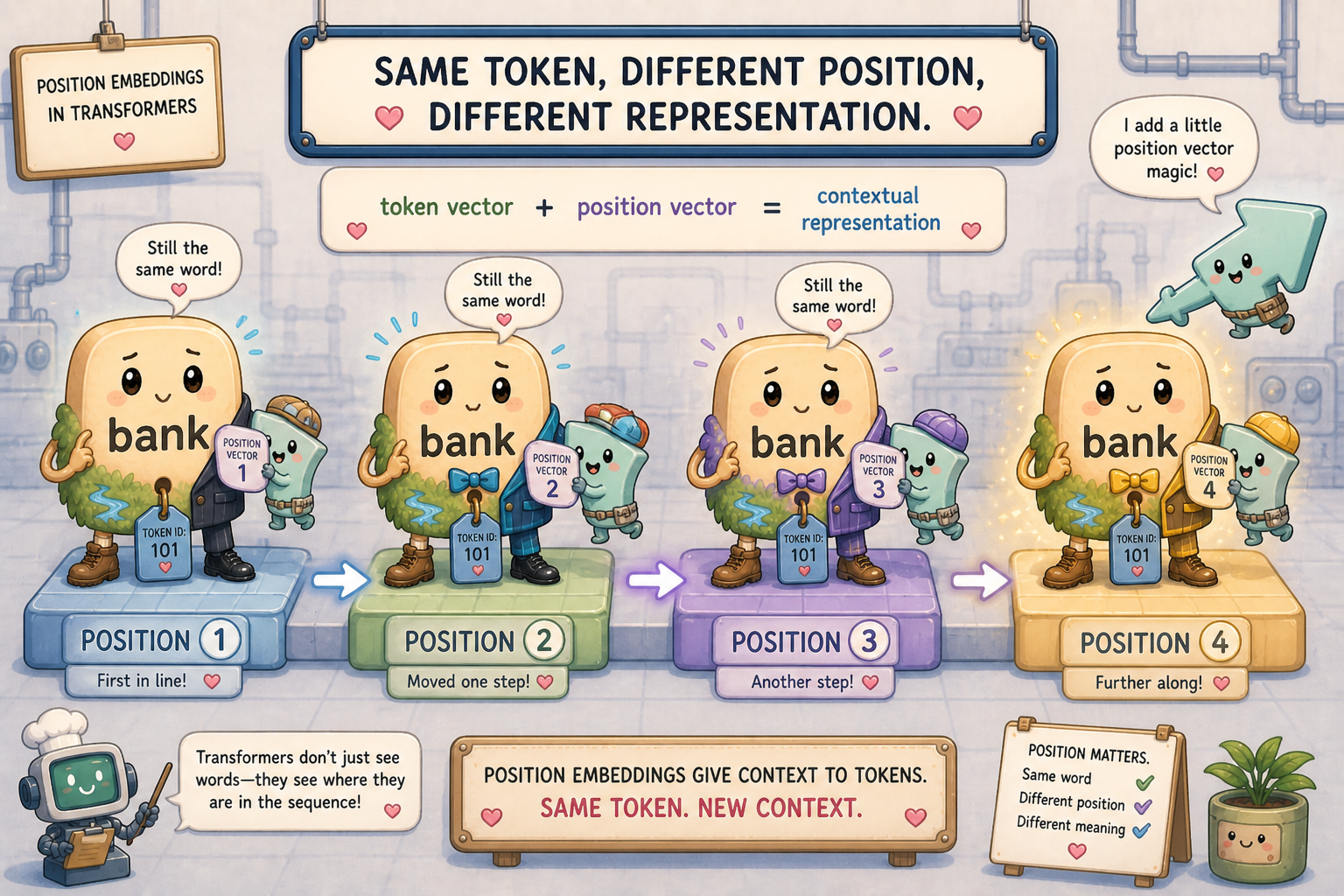
There’s one more problem with raw token embeddings: they carry no order. If you take the same token vectors and reorder them, you get the same set of vectors back, just in a different sequence. The model needs to know where each token sits in the sequence.
The fix is to add a position vector to each token’s embedding. Continuing the sample 2D example:
token vector for " bank" at position 5: E[5] = [1.0, 2.0]
position vector for slot 5:             P[5] = [0.3, -0.1]
layer-0 input:                          [1.3,  1.9]
Vector addition is elementwise:
[1.0 + 0.3, 2.0 + (-0.1)] = [1.3, 1.9]
The same token at a different position lands somewhere different in embedding space. That is the whole trick: later layers now get position information they can use to tell “the bank approved” apart from “approved the bank”, instead of seeing only an unordered bag of token vectors.
W_p = model.transformer.wpe.weight.detach().numpy()  # (1024, 768)
token_ids = tok.encode("I deposited cash at the bank")
i = 5  # position of " bank"
layer0_input = W_e[token_ids[i]] + W_p[i]
Takeaway: the input to layer 0 is token embedding plus position embedding. Each token now has a vector that reflects what it is and where it is, but it still has no idea what’s around it. That’s attention’s job.
Self-Attention: Tokens Look at Each Other

Self-attention is where tokens stop being independent and start sharing information. Coming in, every token has a vector that knows what it is and where it sits, but nothing about its neighbors. Coming out, every token has a vector that has been blended with information from the tokens it cares about. That blend is a major part of how the model eventually tells the financial “ bank” apart from the river “ bank”, though it isn’t the whole story: residuals, output projections, FFNs, and other heads and layers also contribute.
I’ll walk through one full attention sublayer using “I deposited cash at the bank” as the running example. To keep the arithmetic on the page, the worked numbers use a sample 2D version of the math. The real GPT-2 small attention uses 768-dim vectors split across 12 heads, but the shape of the argument is the same.
Step 1: Layer Input
At the start of layer L, every token has a 768-dimensional vector x_i (a list of 768 floating-point numbers). For layer 0 that vector is the token embedding plus the position embedding from the previous section. For deeper layers it’s whatever the previous layer produced. Stack the per-token vectors as rows of a matrix X with shape (seq_len, 768), and the whole sentence rides through attention as that single matrix.
import torch

enc = tok("I deposited cash at the bank", return_tensors="pt")
with torch.no_grad():
    out = model(**enc, output_hidden_states=True)

# Hidden state coming INTO layer L (here L = 11, the last block).
# hidden_states[i] is the input to block i for i in 0..11; hidden_states[12] is
# the output of the last block AFTER the final layer norm (ln_f) is applied.
X = out.hidden_states[11][0]                  # (seq_len, 768)
print(X.shape)                                # torch.Size([6, 768])
Step 2: Layer Norm Before the Projections
GPT-2 is “pre-norm”: before doing anything else, it layer-normalizes X. That rescales each token’s 768-dim vector to zero mean and unit variance, then applies a learned per-dimension scale and bias. A big reason is numerical stability: it keeps the dot products downstream from blowing up or collapsing, while the learned scale and bias still become part of the model’s representation.
block = model.transformer.h[11]
X_ln = block.ln_1(X)                          # (seq_len, 768)
Step 3: Project to Query, Key, Value
Three learned linear maps turn each token’s vector into three different roles:
- Q (query): “what am I looking for in other tokens?”
- K (key): “what do I offer if someone is looking?”
- V (value): “what content do I contribute if I’m picked?”
In GPT-2 the three projections are fused into one weight matrix W_qkv of shape (768, 3*768) plus a bias. One matrix multiply produces Q, K, and V all at once, then we split.
For the sample walkthrough, suppose x_bank = [1.3, 1.9] and all three projection matrices are the 2x2 identity. Then:
q_bank = x_bank @ W_q = [1.3*1 + 1.9*0, 1.3*0 + 1.9*1] = [1.3, 1.9]
k_bank = x_bank @ W_k = [1.3, 1.9]
v_bank = x_bank @ W_v = [1.3, 1.9]
So in the sample we have Q = K = V = X. In the real model the three weight matrices are different and learned, so q, k, and v all point in different directions.
qkv = block.attn.c_attn(X_ln)                 # (seq_len, 2304)
Q, K, V = qkv.split(768, dim=-1)              # each (seq_len, 768)
Step 4: Split Across Heads
A single 768-dim attention would force every token to look at every other token through one lens. Multi-head attention slices the 768 dims into n_heads = 12 chunks of head_dim = 64, gives each head its own Q/K/V slice, and lets each head learn its own pattern. One head might track syntax, another coreference, another topic.
n_heads, head_dim, seq_len = 12, 64, X.shape[0]
Q = Q.view(seq_len, n_heads, head_dim).transpose(0, 1)  # (12, seq_len, 64)
K = K.view(seq_len, n_heads, head_dim).transpose(0, 1)
V = V.view(seq_len, n_heads, head_dim).transpose(0, 1)
Step 5: Score Every (Query, Key) Pair
For each head, compute Q @ K.T. Entry (i, j) is the dot product of token i’s query with token j’s key, which is a scalar measure of “how well does token j answer what token i is asking?”.
For the 2D sample with Q = K = X, “ bank”’s row of scores looks like this:
q_bank = [1.3, 1.9]
k_I         = [1.1, 0.0]
k_deposited = [2.0, 1.1]
k_cash      = [2.1, 0.1]
k_at        = [0.0, 1.2]
k_the       = [0.2, 0.0]
k_bank      = [1.3, 1.9]

q_bank . k_I         = 1.3*1.1 + 1.9*0.0 = 1.43
q_bank . k_deposited = 1.3*2.0 + 1.9*1.1 = 4.69
q_bank . k_cash      = 1.3*2.1 + 1.9*0.1 = 2.92
q_bank . k_at        = 1.3*0.0 + 1.9*1.2 = 2.28
q_bank . k_the       = 1.3*0.2 + 1.9*0.0 = 0.26
q_bank . k_bank      = 1.3*1.3 + 1.9*1.9 = 5.30
Higher dot product means the two vectors are well aligned in direction and have enough magnitude to matter, which the model reads as “this key is relevant to my query”. “ bank” likes itself most (5.30) and “ deposited” second (4.69). In our identity-projection sample these scores just reflect which input vectors happen to point in similar directions; in the real model, that’s not because the model “understands banking” but because the q and k vectors the projection layer learned happen to align well for tokens that should attend to each other.
In code, the per-row dot products I just walked through by hand are computed for every (query, key) pair in one matrix multiply. Q @ K.transpose(-1, -2) produces a (12, seq_len, seq_len) tensor: 12 heads, and inside each head a seq_len x seq_len table where entry (i, j) is token i’s query dotted with token j’s key. The “ bank” row I worked out above is just one row of that table, for one head.
scores = Q @ K.transpose(-1, -2) # (12, seq_len, seq_len)
Dot products are also the workhorse operation of 3D graphics. To shade a pixel, the GPU computes things like dot(surface_normal, light_direction) for millions of pixels independently every frame. That hardware (thousands of arithmetic units running small dot products in parallel) turned out to be a near-perfect fit for Q @ K.T, which is just a big batch of independent dot products. The chips that lit up pixels in video games a generation ago are now scoring queries against keys inside transformers.

Step 6: Scale by sqrt(head_dim)
Quick reminder: softmax is the operation that turns a list of arbitrary numbers into a probability distribution that sums to 1, with bigger inputs getting more of the mass. We’ll work through the formula and a numeric example in Step 8; for now you just need to know that softmax is what comes after this scaling step.
Without scaling, dot products in 64-dim space tend to come out very large in magnitude, which pushes softmax into a near-one-hot output (one weight close to 1, all others close to 0) and makes the model hard to train. Dividing by sqrt(head_dim) keeps the scores in a sane range. For the real 64-dim head, sqrt(64) = 8, so each raw score gets divided by 8. For the 2D sample I’ll skip the scale (sqrt(2) ~= 1.41) so the published numbers line up with the rest of the walkthrough.
import math
scores = scores / math.sqrt(head_dim)
Step 7: Apply the Causal Mask
This is what makes decoder self-attention causal. Token i must not see anything at positions j > i, or it could cheat at next-token prediction during training. We set those entries to -inf so softmax assigns them weight zero. (“Decoder-only” additionally means there is no encoder stack and no cross-attention; it’s a stack of causal self-attention plus feed-forward sublayers.)
For “ bank” at position 5 in a length-6 sentence, the mask doesn’t blank anything because everything from positions 0..5 is allowed. For “ deposited” at position 1 the score row would look like:
[s(0), s(1), -inf, -inf, -inf, -inf]
softmax(-inf) = 0, so the future positions vanish from the weighted sum.
mask = torch.triu(
    torch.ones(seq_len, seq_len, dtype=torch.bool), diagonal=1
)
scores = scores.masked_fill(mask, float("-inf"))
Step 8: Softmax to Attention Weights
Softmax along the keys turns each query’s row of scores into a probability distribution over which positions to attend to. Rows sum to 1.
The recipe is softmax(z)_i = exp(z_i) / sum_j exp(z_j). For the “ bank” row [1.43, 4.69, 2.92, 2.28, 0.26, 5.30]:
exp(1.43) ~=   4.18
exp(4.69) ~= 108.85
exp(2.92) ~=  18.54
exp(2.28) ~=   9.78
exp(0.26) ~=   1.30
exp(5.30) ~= 200.34
Z = sum     ~= 343.0
Divide each by Z to get the weights:
I:0.0122,  deposited:0.3174,  cash:0.0541,
at:0.0285, the:0.0038,        bank:0.5841
Those are the sample-walkthrough numbers. The actual GPT-2 small weights for the financial-context “I deposited cash at the bank” sentence (taken from the head that most clearly picks up the financial-disambiguation pattern, which happens to be layer 11, head 8) tell the same story with different numbers: cash 0.4301, deposited 0.3677, bank 0.1345, with the rest spread thin. About 80% of the mass sits on the two financial-context tokens. This is one visible part of the disambiguation story: “ bank” pulls in signal from “ deposited” and “ cash” to lean financial. Attention weights alone don’t prove that this head is doing all the disambiguation by itself; many other parts of the model are contributing too, and we’ll keep meeting them as the walkthrough continues.
weights = torch.softmax(scores, dim=-1) # (12, seq_len, seq_len)
Step 9: Weighted Sum of Values
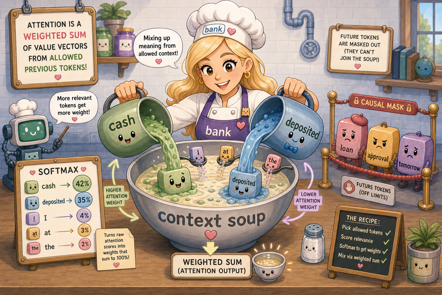
Multiply attention weights by V and sum across the key axis. Each token’s per-head output is a blend of every (allowed) token’s V vector, weighted by how much it attended to them. That blend is context-aware, but it is not the finished representation for the position yet.
For the 2D sample with V = X, “ bank”’s output is computed component by component:
x-component:
  0.0122*1.1 + 0.3174*2.0 + 0.0541*2.1
+ 0.0285*0.0 + 0.0038*0.2 + 0.5841*1.3
~= 0.013 + 0.635 + 0.114 + 0.000 + 0.001 + 0.759
~= 1.52

y-component:
  0.0122*0.0 + 0.3174*1.1 + 0.0541*0.1
+ 0.0285*1.2 + 0.0038*0.0 + 0.5841*1.9
~= 0.000 + 0.349 + 0.005 + 0.034 + 0.000 + 1.110
~= 1.50
So “ bank”’s context blend in this sample head comes out around [1.52, 1.50], shifted from the original [1.3, 1.9] toward “ deposited”’s [2.0, 1.1]. The intuition to take away is this: “ bank”’s blended representation has leaned toward the financial tokens. This is not yet the post-residual vector. It’s just the output of the weighted sum, which still has to go through the output projection (Step 10) and then be added back as a residual delta (Step 11) before the sublayer is done.
head_out = weights @ V # (12, seq_len, 64)
Step 10: Concatenate Heads and Project Out
Glue the 12 heads back into a single (seq_len, 768) tensor and pass it through one more learned linear (c_proj). This is what lets the heads mix; before this step they were operating in isolated 64-dim subspaces. The output of c_proj is the residual delta that will be added back in Step 11.
concat = head_out.transpose(0, 1).reshape(seq_len, n_heads * head_dim)
attn_out = block.attn.c_proj(concat)          # (seq_len, 768)
Step 11: Residual Connection
Add the attention output back to the layer’s input. Residuals keep training stable and let later layers refine the representation rather than overwrite it. After this add, the layer’s “attention sublayer” is done.
For the 2D sample, suppose Step 10’s output projection produced delta = [0.10, -0.30] for “ bank”. Then:
x_after_attn = x_in + delta
             = [1.3, 1.9] + [0.10, -0.30]
             = [1.40, 1.60]
The residual is just elementwise addition. The framing matters: the layer is saying “here’s a residual delta to add to your current vector”, not “here’s your new vector”. That additive framing is what lets you stack 12 of these without the signal exploding or vanishing. (Don’t confuse this [1.40, 1.60] with the Step 9 head output [1.52, 1.50]. They’re conceptually different quantities, computed from different inputs by different operations; I’m using a made-up delta here just to show what the addition looks like.)
x_after_attn = X + attn_out # (seq_len, 768)
Many Heads, Many Layers
The 11 steps above are one full attention sublayer. Steps 5 through 9 (score, scale, mask, softmax, weighted sum) run in parallel across all 12 heads, then Step 10 concatenates and projects, then Step 11 adds the residual. So the heads work in parallel inside the sublayer, not sequentially.
GPT-2 small stacks 12 such sublayers on top of each other, with 12 heads inside each. Different heads learn different relationships, and deeper layers compose the signals from earlier ones into more abstract context.
To make the disambiguation concrete: in “I deposited cash at the bank”, a late-layer head (layer 11, head 8) puts most of its weight on “ cash” (0.4301) and “ deposited” (0.3677). In “I sat on the bank of the river” the same head shifts to “ sat” (0.5728), “ on” (0.1908), and “ the” (0.1624). Note that “ bank” cannot attend to “ river” here because “ river” comes after “ bank” and is blocked by the causal mask. The river signal still informs the model’s predictions at later positions, but the disambiguation of “ bank” itself has to come from the words before it.
Takeaway: attention is the mechanism by which context-free token embeddings turn into context-dependent representations.
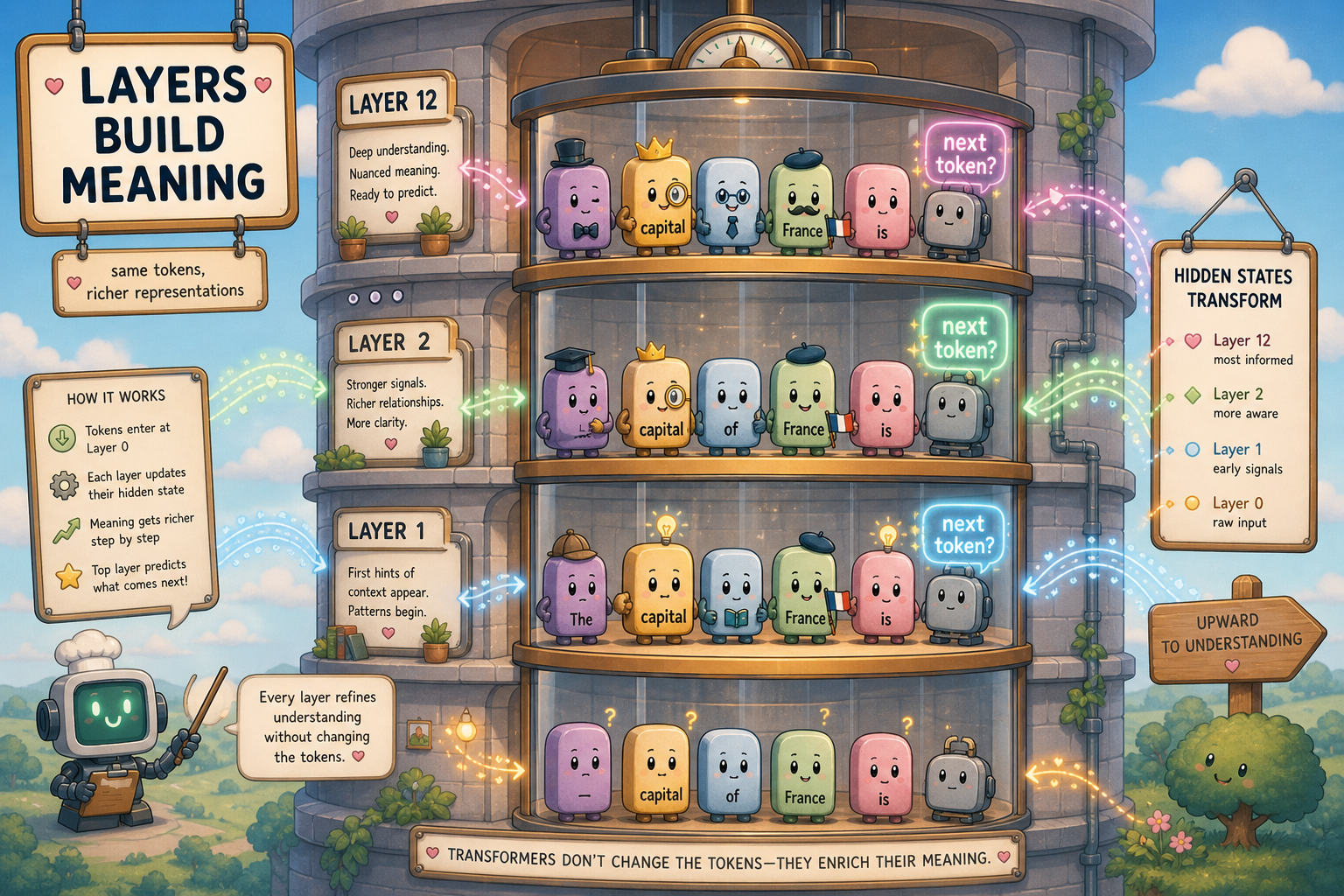
Layers: Building Up Meaning
What a Layer Does
A “layer” in GPT-2 is one attention sublayer (the 11 steps from the previous section) plus a feed-forward sublayer. Each token’s vector at layer L+1 is the layer’s update of its vector at layer L. The attention sublayer is where cross-token mixing happens; the feed-forward sublayer is a per-token nonlinear transform that I’m intentionally leaving out of this post (it’s the focus of a planned follow-up). For now the picture to hold in your head is: at every layer, every token’s vector gets a residual delta added to it based on what’s around it.
Watching Tokens Drift
The forward pass exposes one hidden state per layer, so we can watch a token’s vector move as it climbs the stack. Project the per-layer vectors down to 2D with PCA and you get a literal map of where each token sits at each depth.
from sklearn.decomposition import PCA

text = "The capital of Germany is Berlin. The capital of France is"
enc = tok(text, return_tensors="pt")
with torch.no_grad():
    out = model(**enc, output_hidden_states=True)

# 13 hidden states: embedding output + 12 layer outputs.
# The very last one is post-ln_f rather than the raw output of the last block,
# but it's close enough for visualization purposes.
H = [h[0].numpy() for h in out.hidden_states]   # each (seq_len, 768)

pca = PCA(n_components=2).fit(np.vstack(H))
coords_per_layer = [pca.transform(h) for h in H]
Two things jump out when you actually plot this. First, the two “ capital” tokens start almost on top of each other at layer 0, since they share a token embedding and only differ by their position embedding, but they pull apart noticeably by the deeper layers. The model has stopped treating them as the same word; their contexts are different enough that each one has been pushed in its own direction. Second, the last token’s vector wanders the furthest. By layer 12 it’s sitting somewhere very different from where it started, because it has been accumulating “what should come next?” content from every position behind it.
The Last Position Carries the Answer
That last-position drift is not an accident. At generation time, only the last position’s vector gets used to pick the next token. The earlier positions provide the context that position can attend to; during cached generation, their K/V tensors are what persist and feed the next step. The early layers gather local context, the middle layers blend it, and by the time you reach the top of the stack the last position’s vector encodes whatever the model “thinks” the next token should be.
final_state = out.hidden_states[-1][0, -1] # (768,), already post-ln_f in Hugging Face GPT-2
Takeaway: layers are how the model builds up meaning incrementally. No single layer figures out the answer; 12 layers of residual deltas do.
From Vector to Word: Logits and Decoding
Unembedding
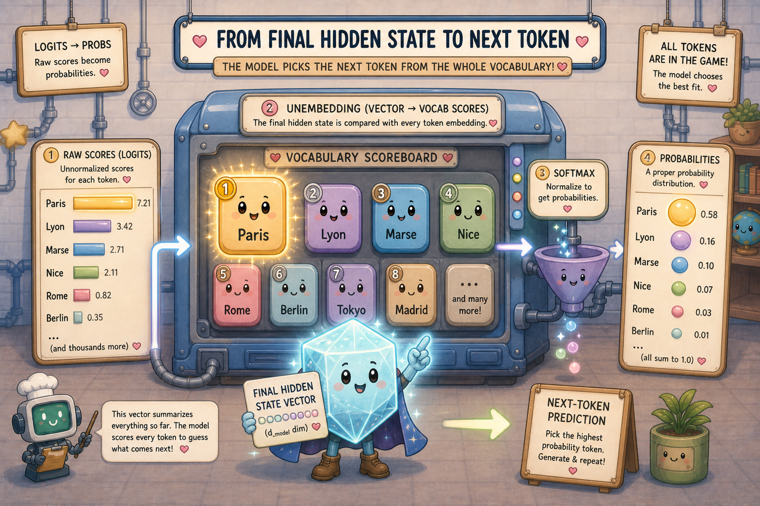
After 12 layers, the last position has a 768-dim vector that’s supposed to encode “what comes next”. We still need to turn that vector into a probability distribution over the 50,257 tokens in the vocabulary. Inside GPT-2’s forward pass, the raw output of the last block first runs through one more layer norm (ln_f) to keep the scale well-behaved, then gets multiplied by the unembedding matrix (the embedding matrix transposed, since GPT-2 ties weights) to get one logit per token, then softmax turns those logits into probabilities. A logit is just the raw, unnormalized score the model assigns to each token before softmax. Bigger means “more likely”, but the numbers are not probabilities yet: they can be negative or larger than 1. Softmax is what squashes them into a proper probability distribution that sums to 1. The unembedding step is the mirror image of the input embedding.
For the sample 6-word vocab and 2D embeddings, suppose the final last-position state is h = [1.5, 1.5]. The unembedding matrix is E.T with shape (2, 6), and the logit for each token is the dot product of h with that token’s embedding row:
logit_I         = 1.5*0.1 + 1.5*0.9 = 1.50
logit_deposited = 1.5*2.0 + 1.5*1.1 = 4.65
logit_cash      = 1.5*2.1 + 1.5*0.1 = 3.30
logit_at        = 1.5*0.0 + 1.5*1.2 = 1.80
logit_the       = 1.5*0.2 + 1.5*0.0 = 0.30
logit_bank      = 1.5*1.0 + 1.5*2.0 = 4.50
Same softmax recipe as in attention: exponentiate and normalize. The token whose embedding row has the largest dot product with h (and therefore the largest logit) gets the highest probability.
On the real model, “The capital of Germany is Berlin. The capital of France is” gives:
enc = tok("The capital of Germany is Berlin. The capital of France is",
          return_tensors="pt")
with torch.no_grad():
    logits = model(**enc).logits[0, -1]       # (50257,)
    probs = torch.softmax(logits, dim=-1)

top_probs, top_ids = torch.topk(probs, 5)
for p, i in zip(top_probs, top_ids):
    print(f"{tok.decode([i]):>10s}  {p.item():.3f}")
#     Paris  0.716
#     Marse  0.056
#      Lyon  0.053
#     Stras  0.026
#      Nice  0.021
More than 70% of the probability mass is on “ Paris”, and the next few candidates are mostly tokens that begin other French city names. The model is not “looking up” Paris in a table; the only reason this works is that 12 transformer layers (attention plus FFN) have moved the last position’s vector into a place where its dot product with the “ Paris” row of the unembedding matrix is the largest logit in the vocabulary.
Greedy vs Sampling
Once you have the probability distribution, you still have to pick a single token. The two basic options:
- Greedy: take the argmax (the index of the highest-probability token, the “winner” of the distribution). Deterministic, gives the same output every time for the same prompt.
- Sampling: draw a token weighted by the probabilities. This is why the same prompt can give different answers on different runs.
There’s also temperature, which scales the logits before the softmax. Low temperature sharpens the distribution (more peaked, more deterministic-looking). High temperature flattens it (more variety, more wild outputs). Temperature 0 is effectively greedy.
def next_token(logits, temperature=1.0, sample=False):
    logits = logits / max(temperature, 1e-6)
    probs = torch.softmax(logits, dim=-1)
    if sample:
        return torch.multinomial(probs, num_samples=1).item()
    return int(torch.argmax(probs))
Stopping
The model needs some way to decide it’s done. The standard approach is a special end-of-text token in the vocabulary: if the next token is EOS, stop. Otherwise, hit a max-length cap so generation can’t run forever. Real chat systems layer more on top: configurable stop sequences, tool-call boundaries that hand control back to a runtime, server-side token limits, and policy or safety stops that can cut a generation short.
if next_id == tok.eos_token_id or len(generated) >= max_new_tokens:
    break
Takeaway: turning a vector back into a word is just one more matrix multiply plus a softmax. Everything that makes a chatbot’s output feel “smart” or “creative” is choices made on top of that distribution.
The Loop: Autoregression
One Token at a Time
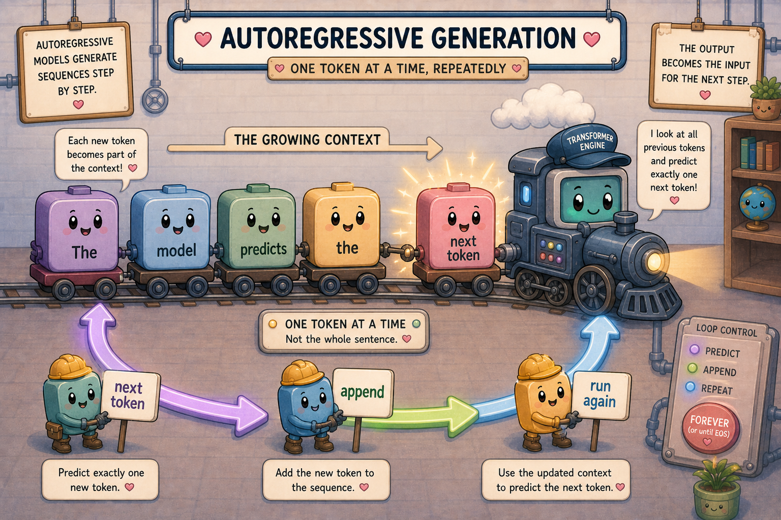
The whole generation procedure is now just a for loop. Pick the next token, append it to the prompt, run the forward pass on the longer sequence, repeat. That’s it. There is no separate “generation” mode, no extra component that knows how to produce sentences. The same forward pass that gave you “ Paris” gives you the token after “ Paris” once “ Paris” is part of the input.
ids = tok.encode("The capital of Germany is Berlin. "
                 "The capital of France is")
for _ in range(10):
    with torch.no_grad():
        logits = model(torch.tensor([ids])).logits[0, -1]
    next_id = int(torch.argmax(logits))
    ids.append(next_id)

print(tok.decode(ids))
# The capital of Germany is Berlin. The capital of France is
# Paris. The capital of the United States is Washington
Conceptually, each step reruns the entire forward pass on the entire sequence so far. In practice, production systems use KV caching: the K and V tensors at every layer for previous tokens are stored and reused. On each new step, the model computes the new token’s Q/K/V, appends its K/V to the cache, runs its attention against the cached K/V, applies the rest of that token’s layer work, and computes the final logits. That is much cheaper than recomputing the full sequence, and in eval mode it gives the same next-token distribution apart from tiny implementation-level numerical differences.
The core text-generation model in mainstream chatbots is usually some scaled-up version of this autoregressive decoder loop. Architectures and serving stacks differ in the details, but the shape of the inner loop is the same: a transformer-based decoder, run autoregressively, one token at a time.
Why It Feels Smart
Inside this simplified core decoder pass, there’s no clever planner, no goal-tracker, no module that “decides what to say”. At every step the model has spent its transformer layers (12 of them in GPT-2 small) refining the last position’s vector based on everything before it, scored every token in the vocabulary against that vector, and then the decoding strategy picked one. The “intelligence” lives in the layer weights, not in any single forward step. What you experience as a coherent response is just that loop running thousands of times, each step nudged by all the steps before it. (Production chat products wrap this core loop in a lot more: retrieval, tool use, safety systems, reasoning and agent scaffolding. Those layers can absolutely look like planning, but they sit outside the decoder itself.)
Takeaway: autoregressive generation is a for loop. Everything interesting about it comes from the model inside the loop, not from the loop itself.
Things I Skipped
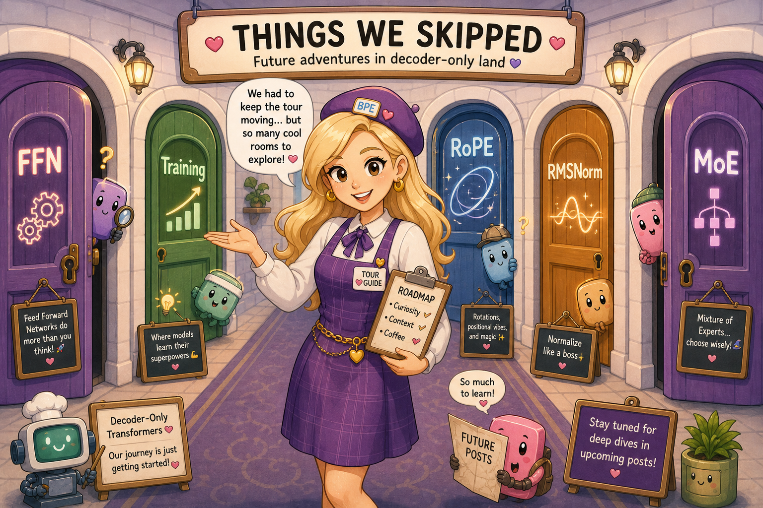
To keep this post focused, I left out a few topics. I’ll write follow-up posts on these later:
- The feed-forward sublayer inside each layer. It’s a big chunk of the parameters and it’s where a lot of the model’s “knowledge” appears to live. I’m saving it for a dedicated follow-up post.
- Training. Everything above is about inference, what happens once the weights already exist. How those weights got learned (loss function, backprop, optimizer, data) is a different post.
- Modern variants. GPT-2 small is a good teaching model, but production LLMs differ in the details: rotary position embeddings (RoPE) instead of learned position vectors, grouped-query or multi-query attention instead of plain multi-head, mixture-of-experts FFNs, RMSNorm instead of LayerNorm, and so on. The basics don’t change, but the specific machinery does.
Summary
The whole pipeline in one paragraph: prompt -> tokenize into integer IDs -> embed each ID and add a position vector -> run the model’s transformer layers (12 in GPT-2 small) of attention and FFN, each one nudging the per-token vectors a little -> read off the last position’s vector -> apply a final layer norm -> multiply by the unembedding matrix to get logits -> softmax to get probabilities -> sample or argmax to pick the next token -> append to the prompt -> repeat until EOS or a length cap. That’s an autoregressive decoder-only transformer. The core text-generation model in mainstream chatbots is usually some scaled-up, polished-up version of that loop, wrapped in retrieval, tools, safety systems, and other scaffolding on top.
Comments